How to use dynamic array in VBA / macro

Sorry Pravin to keeping your query waiting. You asked me a query about how to use dynamic array in VBA but in my last post I explained about basic use of array but my blog is for all the readers ;-).

So here we go, We get into such scenario where we actually doesn't know what length of array we would need in our program and here dynamic array helps you. Lets check a example program:

Ex1:

Sub MyDynArray ()

Dim MyArr() as integer, iArrLenghth as Integer, iCntr as Integer

iArrLenghth =  Sheet1.Range("A1").End(xlDown).Row

Redim Preserve MyArr( iArrLenghth-1)

For iCntr = 0 To iArrLenghth
   MyArr(iCntr) = Sheet1.Range("A" & iCntr+1)
Next iCntr

For iCntr = 0 To Ubound(MyArr)-1
   If MyArr(iCntr) = 5 Then
        MsgBox "Number 5 found"
        Exit For
   End If
Next iCntr

End Sub

In example code is storing all numbers in column A of sheet1 to an Array variable and then searches in array for number 5 and throws message if number 5 found and ends.

In example procedure at first line I have declared dynamic array with other variables

Dim MyArr() as integer, iArrLenghth as Integer, iCntr as Integer

while declaring dynamic array we doesn't specify its length.

Next line I get count of rows having data in column A of sheet1 into variable.

iArrLenghth =  Sheet1.Range("A1").End(xlDown).Row

At next line we set length of array variable at runtime so if column A has 5 rows of data then Array's length would be 0 to 4.

Redim Preserve MyArr( iArrLenghth-1)

Here we can also use only Redim no need to use Preserve keyword.

Preserve is required only if we have data stored in array and we do not want to loose it.
If our array is having some data stored and if we do not use Preserve keyword as shown below then all stored data will wipe out.

Redim MyArr( iArrLenghth-1)

Next I have use a for loop to store value from column A of sheet1 to array variable

For iCntr = 0 To iArrLenghth
   MyArr(iCntr) = Sheet1.Range("A" & iCntr+1)
Next iCntr

After that I have used another fir loop which I am using to loop through all elements of array variable and to find if any element is having value as 5 and if found then exit loop.

For iCntr = 0 To Ubound(MyArr)-1
   If MyArr(iCntr) = 5 Then
        MsgBox "Number 5 found"
        Exit For
   End If
Next iCntr

Here I have used inbuilt function UBound() which gives length if array. and I have used Exit For which get use to terminate For loop.

So here are some basics which will help you to manipulate  data in array and access to flexible array length.

Let me know in case of any queries.

Thanks

.

How to use VLOOKUP Formula in Excel 2003 , 2007

Hello Readers,

I have added one post about for a formula which really helped me a lot in my MIS work.

The most useful formula in excel is VLOOKUP for MIS guys. .

many guys find difficulty to learn this formula.So Lets go step by step I will show you some easy examples.

Before learning the formula we should know that what is the use of the formula.

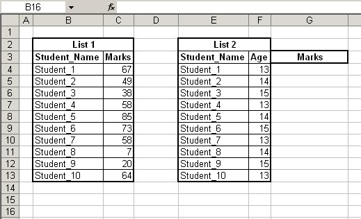
This formula is very useful when you have to find out value from a list, say there are two lists One with 2 columns Student_Name & Marks And another table Student_Name & Age As shown in the Image.

So with the help of VLOOKUP formula we can find out Marks in column G for Students Given in Colomn E

As shown in below image

We can see the entered formula in cell G4 "=VLOOKUP(E4,B3:C13,2,0)"

The formula has divided into the 4 parts.

= Vlookup(Lookup _value, Table Array,Column_number,Range_Criteria)

1. Lookup Vaue which is E4 (means which value we are going to find in List 1 )

2.Table array B3:C13 (You have to select total List1 )

3.Column number (Which coumns you want as output, as you can see there are 2 columns in List 1)

4.Rage ( It should be "0" or "FALSE", We will disscuss on same later on )

So now you have understood what we have to entered into each part of the Formula.

Let understand what actually the formula does .

1. Lookup Vaue which is E4 (means which value we are going to find in List 1 )

Formula first take Lookup Value and find lookup value in first column of Table Array

Means it actually finds "Student_1" in Column "B3:B13"

It get value "Student_1" in cell B4

after that it checks Column number (which we have given 2 in the formula).

And as B4 is column 1 of table array so 2 would be D4 and D4 is marks of Student_1

In such way it find out marks of Given Lookup Value

Questions!!!!

What happens when Formula doesn't find Lookup value in first column of table array ??

this is nice question, The formula simply gives Error of Not Found like this => "#N/A"

If you want to test you just change Lookup value means E4 to "Student_11" as Student_11 is not in the List1 it will show #N/A error

But its just a one result what for other marks for List2 ???

Now as you have created the formula you need not write it again in every cell Just copy cell G4 and Paste into Where you want to apply the formula That is G5:G13.

Isn't it easy ????
Formulas are just 10% of total excel power if you want to unleash the power of MS-Excel then start learning VBA. I would recommend to join a course which is prepared for absolute beginner such as :
Excel VBA MACRO Kick-start Course for absolute beginner

Be familiar with Excel

Following are some tips

SPLIT WINDOWS AND FREEZE PANES

In excel you would need to use splitting function because Splitting a window allows you to work on multiple parts of a large spreadsheet simultaneously and Freezing the pane allows you to always keep one part of the spreadsheet (e.g., column or row labels) visible.

To use this function Drag the split horizontal and split vertical icons to the desires positionsClick on the freeze pane icon from the tool bar to freeze the panes

HIDE AND UNHIDE COMMAND

Hide and unhide function in excel Allows you hide and unhide particular rows or columnsSimplifies working with the spreadsheetPrevent certain information from being seen
To use hide and unhide Select the row(s) or column(s) to be hidden/unhiddenSelect Format : Row : Hide/Unhide or Format : Column : Hide/Unhide
MOVING AROUND A SPREADSHEET WITH CTRL, SHIFT, AND ARROW KEYS

It saves your lots of timeMove the first or last cell of a contiguous data block without scrolling

To use scrollfree movement use following keys

Ctrl-Arrow : Move to the first/last data cell in the arrow direction

Ctrl-Shift-Arrow : Selects the cells between the current cell and the first/last data cell

NAME CELLS/RANGES

Why to use :
Allows specific cells or cell ranges to be referred to by name
Allows you to write equations such as = Quantity*Cost instead of =$B$12*$C$4

How to Use:

Select the cell or cell rangeSelect Insert : Name : Define from the menu bar

SORT COMMAND

Use :

Correctly sorting a series of rows or columns without disassociating the data is critical to many modeling efforts

how to use:

To sort by single category, just click into column, NEVER highlight column (would destroy table integrity)To use multiple criteria, click any cell of data table, select Data…Sort Data table will be selected